How To Sum a Column in Google Sheets?

The SUM function in Google Sheets allows you to display the total of selected cells. But it is not just a feature to make simple additions. To effectively use this function, you would need a dedicated cell where you can display a sum of cells above in the same column or from a different column.

There are multiple ways to use this feature. The most common is typing SUM and then mentioning the range of cells you want to have a sum of. But did you know that you can drag the range of cells or the whole column with the cursor instead of typing the range of cells manually?

That is exactly what we are here today for. In this article, I’ll discuss four different methods, of course, apart from the usual method of typing SUM.

Let us get into it.

Ways To Total a Column in Google Sheets

To make things simpler, Google Sheets has a formula bar right above the cells and below the ribbon bar. If a cell is displaying a sum or a total and you have no idea where that cell fetches the number from, then you can simply click on the cell and see its formula from the formula bar.

Needless to say, you can also write your own formulas directly into the formula bar, and it will work the same way. Below are four ways to perform the addition of an entire column in Google Sheets.

Method 1: Using the SUM Function

To use the SUM feature, you have to write the whole formula down. There are multiple ways to add cells or a range of cells into the sum formula.

You can even sum a whole column up using the same feature. Here are some examples of using the SUM feature in Google Sheets.

• Individual cells: =SUM(A1, A2, A3)
• Range of cells: =SUM(A1:A5)
• Whole column: =SUM(A:A)

Method 2: Using the Status Bar

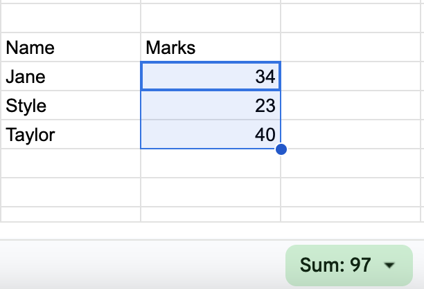
The status bar at the bottom shows smart suggestions like summing up the selected range of cells. The status bar by default, does not show any action or suggested feature.

But once you select a range of cells that contains numbers, it suggests the SUM feature by default on the bottom right.

All you have to do then is to check out the sum shown in a green box in the status bar, here is a step-by-step guide for it:

1. Select the first cell of the range.
2. Press shift and select the last cell of the range.
3. If you want to total a whole column, then click on the head of the column.
4. Now check out the bottom right corner of the screen on the status bar.
5. There will be a sum of your selection in a green box with the text “Sum: “

Method 3: Using Function

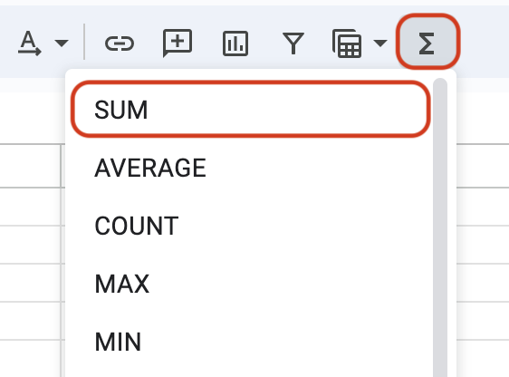
The function button, as the name suggests, performs a few functions. The first one of these functions is the addition or the sum function.

You will see the addition or summed display upon selecting a range or the whole column and using the function feature to display the summed numbers.

Here is how you can perform the addition or sum using the Function button:

1. Select the first cell of the range.
2. Press shift and select the last cell of the range.
3. If you want to sum up the whole column, then click on the head of the column.
4. Locate and click on the Function button that looks like “Σ”.
5. It will show the formula on the cell below the selected range or in the first cell of the column if you have selected the whole column.
6. Press enter to apply that formula.

You will now have the sum of the selected cells or the whole column.

Method 4: Using Drag & Drop

AutoSum is a great feature where you can do a sum of columns or a selected range of cells with the help of just one button. The only unfortunate thing is that this button and the feature of AutoSum are only available in Excel.

While Google Sheets does not have a default feature or a button like AutoSum, it does, however, have a way around to do the same thing. Here is how:

1. Select any empty cell in a column below the cells with numbers where you want to perform the sum or addition.
2. Apply the SUM function in the cell by writing =SUM(cell1, cell2, cell3), or if it’s a range of cells, then simply write =SUM(cell1:cell10).
3. Now drag the edge of this cell to the next cell below the next column or to all the adjoining cells below the columns.

Dragging the edge of the cell to the next cell will copy its formula and replace the cell identification with the relevant cell.

This way, you only have to write the sum formula once and drag the cell across to sum other columns as well.

Method 5: Using Conditional Formatting

The SUMIF or conditional formatting technique is an advanced version of the SUM feature. As the name suggests, SUMIF is an amalgamation of SUM & IF. It can be used in transposing Google Sheets as well.

This feature will only perform the sum of the selected range based on specific criteria. The format of the SUMIF feature contains a range of criteria, the criterion, and the range of cells.

For instance, if you have three columns containing names (A), date (B), and amount donated (C) for a cause, and if you want to churn out how much a particular individual has donated, then you have to mention the range for criteria which is all cells containing names, mention the criterion with text and the range of cells which you want to sum.

It will be something like: =SUMIF(A2:A50, “[Name]“, C2:C50)

It’s quite similar to count if not empty. That said, you can also integrate third-party tools like add-ons to explore the possibilities of Google Sheets further.

For instance, there are many add-ons for the AutoSum feature that are present in Excel but not available on Google Sheets.

Frequently Asked Questions

Wrap Up!

That’s all to get the sum of a column. The feature, especially with its advanced version of SUMIF, is a great tool for creating and maintaining complex numerical.

Once you have assigned the SUM formula to designated cells, all you have to do then is to change some numbers on some cells and the SUM feature will reflect the changes.