As a frequent Google Sheets user, I understand how frustrating those gridlines can be. While they’re useful for organizing the data, they can also look cluttered and messy. If you want to remove them, let me help you out.
The gridlines in Google Sheets can be removed either from the entire sheet or specific cells. Not just removing but I’ll also walk you through how to customize it, enabling you to format your Sheets like a pro.
Steps to Remove Gridlines in Entire Google Sheet
Gridlines can sometimes interfere with the readability of your data, especially when you’re adding a line graph, a pie chart, statistics, or other visual elements. Follow the steps below to remove them from your entire sheet:
- Open the sheet you’re working on.
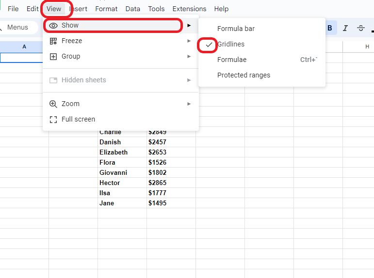
- Find “View” from the top bar.
- On the dropdown, choose the “Show” option. It will open a sub-menu.
- Untick the “Gridlines” option as shown in the screenshot below.
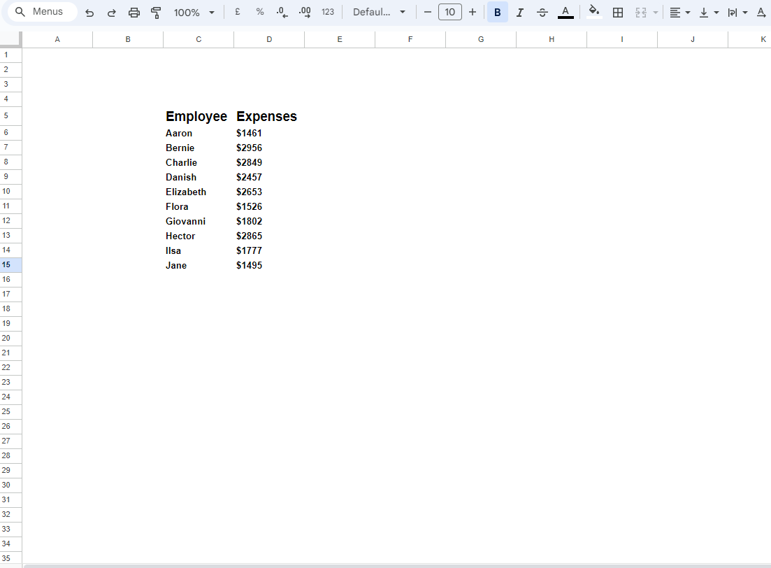
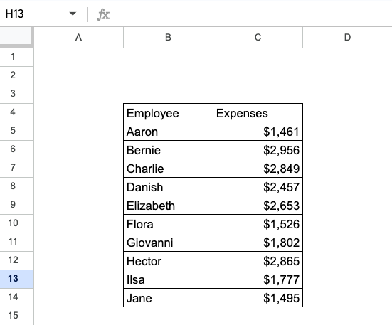
- This will remove all the gridlines from the sheet you’ve selected. It would look like this:
Steps to Remove Specific Gridlines in Google Sheets
In case you want to highlight specific cells with lines and get rid of the lines from the rest of the sheet, the method is slightly different. Here’s how to do it:
- Open the sheet you want to edit.
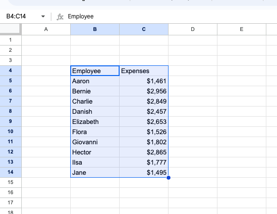
- Select the cells or range you want to highlight. (Feel free to choose according to your requirements).
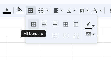
- On top of the Google Sheets, right below the menus, you will find a list of shortcut icons. Choose the one that says “Borders”.
- From the “Borders” submenu, you’ll see various types of border options. Choose the appropriate type of border for your selected range.
- Once you’ve set the borders, go to “View”, select “Show”, and remove the checkmark next to “Gridlines”. This will leave gridlines only on the selected range.
Want To Print Google Sheets Without Gridlines?
When you take printouts straight out of Google Sheets, all the gridlines appearing on the entire sheet, instead of the highlighted data are bound to make your print look messy.
In case you want them gone when you are only taking the printouts without changing the settings inside the sheet. Let me show you how:
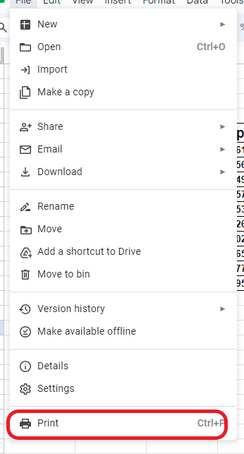
- In the top left corner of the menu, Choose the first option “File”.
- Scroll down to the bottom of the menu and Select “Print”. This will take you to the print settings.
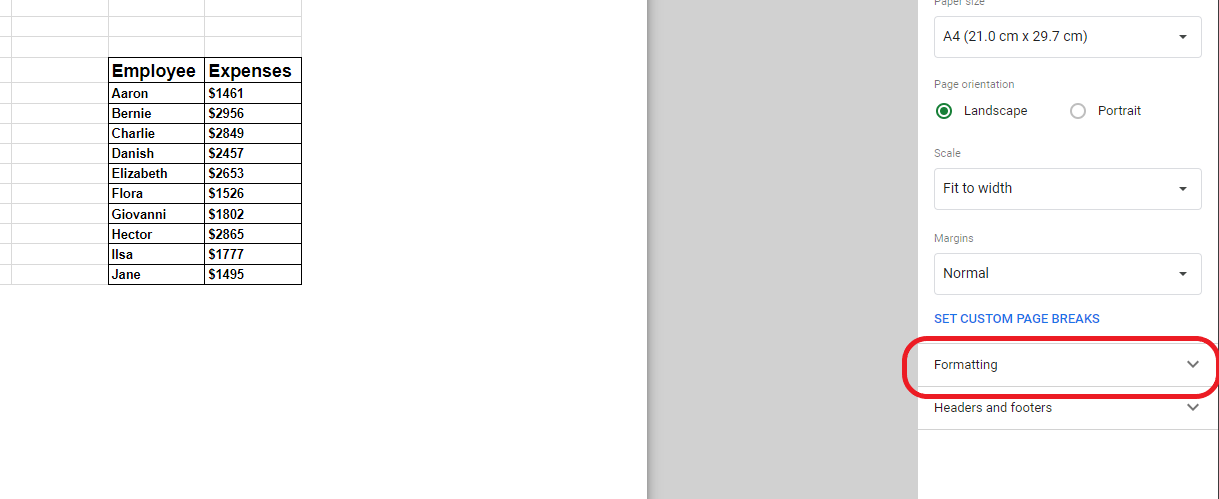
- You can adjust various print settings, including the size, and orientation, and set custom or prefixed margins. Make sure they align with the requirements and proceed to the section below.
- Now, click on the formatting.
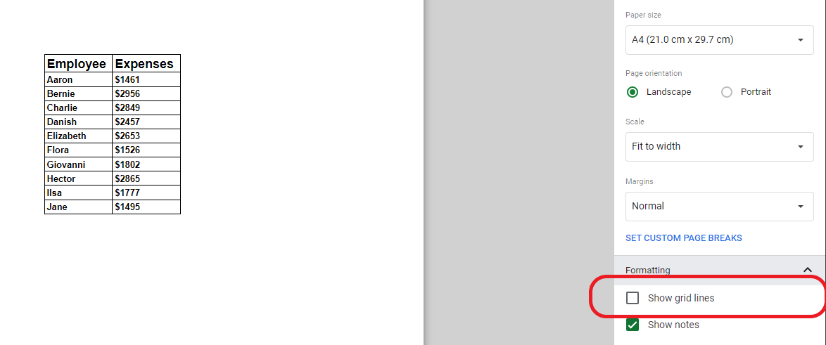
- By default, you will find the gridlines check box ticked. Uncheck the box to remove the gridlines in the printed document.
- Click “Next” to preview the print setup. Once you’ve cross-checked the details, click on the print button to send the request to the printer.
Frequently Asked Questions
You can hide borderlines in a Google sheet using a list of shortcut icons appearing below the main menu. Select the range of cells and choose none. This will take away any borderline you might find.
Go to the View tab from the main menu and click on Show. Look for a tickmark that corresponds to the gridline. If you don’t tick, click on the gridlines. This will add gridlines to your entire sheet.
Yes, you can do so using the mobile app as well. Scroll down to the bottom left corner of the sheet, which displays the sheet name. Click on the menu. You will find a toggle on/off bar that says gridlines. Switch it to off, the gridlines will go away.
Select the cells or the range where the gridlines are appearing. Set the border to none. Now click on the top left cell and select the entire sheet. Click on view, go to show, and untick the gridlines.
No, removing the gridlines will not affect the data in your spreadsheet. Although it might be difficult to identify or input data on a specific row or column.
Wrap Up!
As a beginner, navigating through Google Sheets can be overwhelming due to the multitude of options available. Even basic tasks like removing gridlines can be challenging. Hopefully, this guide helped you get rid of it.

Leave a Reply