Do you have a list of dates as to when a certain set of tasks were performed, and want to summarize the data by period for a project? The quarter is one such range, corresponding to three months.
Be it financial planning by comparing performance across various periods, presenting data precisely, performance reviews or forecasting models, calculating quarters comes quintessential. By mastering the simple yet powerful function of Excel, you can elevate the effectiveness of your data-driven strategies.
I’ll guide you through the step-wise process. Without further ado, let’s dig in!
Steps To Calculate Quarter from Date
For this, you must use the ROUNDUP function together with the MONTH function.
Here’s what the formula looks like:
=ROUNDUP(MONTH(cell/3,0)
Let’s understand the method with an example.
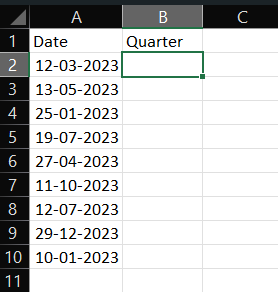
- Consider the following data to use.
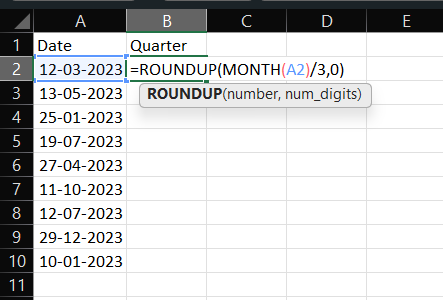
- Now it’s time to calculate the Quarter for each date, so put down the following formula: =ROUNDUP(MONTH(A2)/3,0) into cell B2.
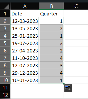
- Then press Enter. You’ll see “1” as a response to the function.
- Drag the autofill handle down to apply the formula to the below cells (B3 to B10).
Now that you’ve calculated the quarter for a respective date, it’s much easier to make financial decisions.
Alternative Method
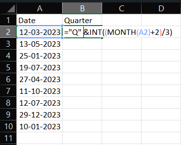
- In the blank B2 cell, type in the following formula: =”Q” &INT((MONTH(A2)+2)/3).
- Then press Enter.
- Drag autofill handle down to apply the formula to the below cells (B3 to B10).
Other Functions To Know
If you have more than a year of data, just using the formula to obtain the quarter for a corresponding gate can create even more confusion. Converting date into quarter and year in this case, can come in handy.
Here’s how you can do it:
- For this, I will use a new set of data.
- On the blank B2 cell, type the formula as follows: =”Q” &INT((MONTH(A2)+2)/3) & “-” & YEAR(A2). Then, press Enter.
- Now drag down to apply the formula to the below cells (B3 to B10).
Converting Date into Full Quarter Name and Year
There’s also a formula with which you can convert into full quartern name and year. The formula is not very different from showing quarter & year, and it looks like this:
=”Quarter ” &INT((MONTH(A2)+2)/3) & ” ” & YEAR(A2)
- In the same dataset, replace the above formula with the one provided and press Enter.
- Drag down to apply the formula to the below cells (B3 to B10).
Apart from finding a quarter from the date, you can do several other things in Excel. For instance, you can separate the date and time, find IQR, calculate the Median If, and more.
Frequently Asked Questions
To convert a date to the nearest quarter in Excel, type the formula “=ROUNDUP(MONTH (A1)/3,0), and press Enter.
Instead of the date, if the input is the month name, we must compare it with a list of months to determine the sequence number of the feeding section. The formula looks like this: =CHOOSE(ROUNDUP(MATCH(A1, {“Jan”,”Feb”,”Mar”,”Apr”,”May”,”Jun”,”Jul”,”Aug”,”Sep”,”Oct”,”Nov”,”Dec”})/3,0),”Q1″,”Q2″,”Q3″,”Q4″)
To combine year and quarter in Excel, apply the formula: =”Q” &INT((MONTH(A2)+2)/3) & “-” & YEAR(A2). Then, press Enter.
Wrap Up!
Excel doesn’t have a QUARTER function, so a quarter is typically calculated using formulas based on the MONTH function. It might come in handy to analyze the financial data of a business, but the formula provided is based on calendar quarters instead of fiscal quarters, which many businesses follow.
Saying that comes an end to my guide. I hope the above guide helps. I will see you in another such informational guide. Till then, goodbye and take care!


Leave a Reply