The Complete Guide To Google Sheets Not Equal Operator

The “Not Equal” operator in Google Sheets is quite versatile and can be used in multiple scenarios like data validation, filtering, conditional formatting, finding non-matching values, removing duplicates, and more.

In other words, becoming adept with this operator might result in a 10-20% improvement in your overall capability when working with spreadsheet data. That’s where this guide comes in.

In the subsequent sections, I have explained everything there’s to about it. I also shared some practical examples for easy understanding.

So, without further adieu, let’s dig in!

Not Equal in Google Sheets: Explained

In Google Sheets, “<>” represents “not equal” and is placed between two values, calculations, or cell values. Alternatively, you can use “NE” to do the same.

As in the name, it’s primarily used to validate if the values in respective cells are equal or not. For example, =A1<>B1, and the values in the respective cells are compared. That’s not it.

The function also finds its use in conditional formatting or filters. For instance, if you want to highlight values that are not equal to zero, just type in A1<>0.

You can also use it to count/sum non-matching values and remove duplicate values. So, let’s start learning its practical use.

Not Equal Symbol and Formula Construction

1. Compare

The “Not Equal or <>” formula in Google Sheets is constructed as =Value1 <> Value2.

Here, my motive is to compare Value1 and Value2 and find out whether they’re equal or not.

So, as you press Enter, Google Sheets undertakes the task and displays the results as “TRUE” if the values are not equal or “FALSE” if they are. Count if not blank is one of its key examples.

2. Filtering Data

The formula to filter data/dataset using the Not Equal function is constructed as follows:

= FILTER(Value1:Value3, Value2:Value3 <> “Data”)

Here, I want to determine which cells in the Value 2 and Value 3 columns don’t have the specified value or data.

So, Value 1:Value 3 is the space where you want Sheets to evaluate, and Value2:Value 3 is the last column in the space.

Once I press Enter, Google Docs will evaluate and segregate the data that doesn’t match the provided condition.

P.S.: For numerical data, remove the “”, it’s only applicable for ones that contain words.

3. Count Data

Here, you need the COUNTIF function in conjunction with the Not Equal to count the number of cells in a range that are not equal to a specified criteria.

Here, the formula is constructed as follows:

=COUNTIF(Value1:Value2, “<>” & Data)

Value1: Value2 is the range of data you wish to evaluate, and data is the data you want to exclude. In layman’s terms, you want to count the number of values from Value1 cell to Value2 cell that aren’t equal to data.

So, as you press Enter, Google Sheets counts all the values and displays the result.  

4. SUM Function

While this is primarily used to total a column, cell, or range of cells, you can use it with not equal operator.

If you want to add the values in a cell excluding a few, the Not equal function comes in handy, and the formula is constructed as follows:

=SUMIF(Value3:Value4, “<>” & Data, Value1:Value2)

Here, the intention is to add the values in the cell range from Value3 to Value4, excluding the ones where the value is equal to “data” in the same range.

So, “Value3:Value4” is the range of cells to check the “not equal” condition, “data” represents the not equal value, and “Value1:Value2” is the range of cells to sum if the condition is met.

5. Compare SUM function

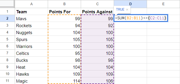
Using the <> function, you can compare the SUM of two sets of data, and the formula is constructed as follows: =SUM(Value1:Value2) <> (Value3:Value4)

Breaking down the formula: Value1:Value2 is the first range of cells, and Value3:Value4 is the second range of cells.

Putting the formula, Google Sheets will sum the total amount from Value1 to Value2 cell and from Value3 to Value 4 cell, and compare the result. If the values are not equal, it will display “TRUE” and “FALSE” if otherwise.

6. Conditional Formatting

You can also use the Not Equal function to conditionally format a set of cells. For example, you want to highlight the cells whose values aren’t equal.

First, select the cells you wish to format, for example, Value1:Value2. Then, in the conditional format rules section, put a formula as follows: = Value3<> Value4, and “Done.”

Each cell in the selected range (Value1:Value2) is formatted where corresponding values in the “Value3” and “Value4” columns are not equal.

Using Not Equal Operator in Google Sheets

1. Compare

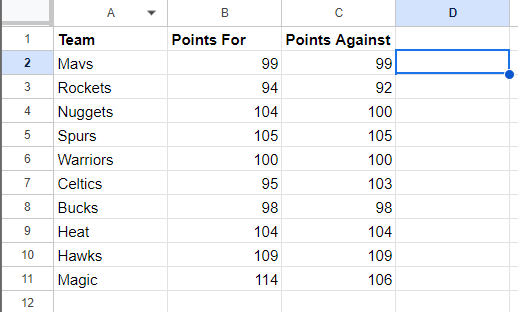
The most common use of the “Not Equal” function is to compare two cells if they are equal or not. Here are the steps to follow:

1. Select an empty cell adjacent to the data set.
   
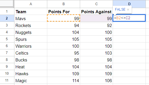
2. Input the “Not Equal” formula: =B2<>C2.
   
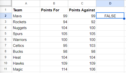
3. Press Enter. If the values of the compared cells are equal, Google Sheets will generate a “False” result and a “True” if not equal.
   
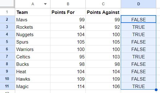
4. Copy down the column to apply the formula to the entire column.
   

2. Filtering Data

This formula lets you sort and filter the data that you see when you view the spreadsheet. This is especially helpful when you’re searching for a specific type of data in a spreadsheet containing thousands of datasets.

Here’s how to do it:

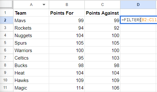
1. In the adjacent empty cell, type the FILTER function and select the range of cells you want to filter.
   
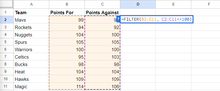
2. In this case, the condition is that the values in columns B and C shouldn’t be equal to “100”. So, complete the formula as =FILTER(B2:C11, C2:C11<>100). Then, Press Enter.
   
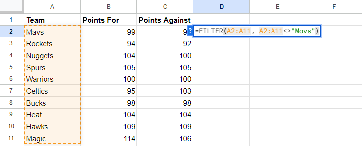
3. For data containing words, just use “” as follows:
   
4. Press enter.

3. Count Data

The Count data with the Not Equal function in Google Sheets lets you tally all the cells with numbers that aren’t equal to a specified criteria. Now that you already know the formula format, let’s understand it by an example.

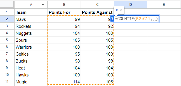
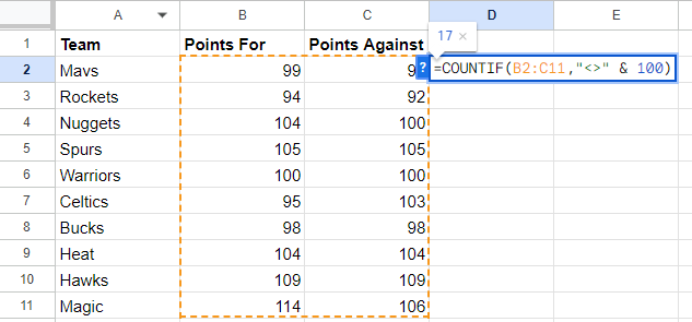
1. In the adjacent empty cell, type in the COUNTIF function and select the number of cells you want to include.
   
2. Then use the not equal function, a double quotation followed by &, and the data you want it not to count. Here’s what the complete formula looks like:
   
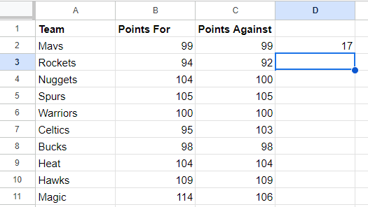
3. Then press Enter and it will show a result.
   

4. SUM Function

Adding a set of data by excluding one or more can get a bit tricky. This is where the “Not Equal” function comes in handy. This is how you can do it:

1. In the adjacent empty cell, write in the SUMIF function followed by the cells where you want to apply the “not equal” criteria. In my case, it was C2:C11.
   
2. Then insert the Not equal function in a double quotation followed by “&,” the excluded data and the cells you want to add. Here’s how the formula looks:
   
3. Press Enter.

5. Compare SUM Function

Often, you might find yourself with two separate sets of data and need to ascertain if sum of their values isn’t equal to one another.

Here’s how you can do it:

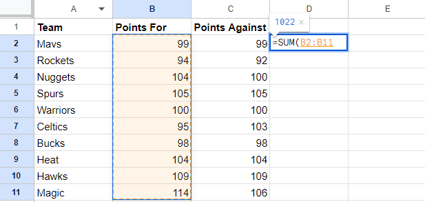
1. In the adjacent empty set, type in the SUM function and select the first range of data.
2. Complete the formula as in the image below.
3. Press Enter.
4. Copy down the column to apply the formula to the entire column.

6. Conditional Formatting

Conditional formatting is a unique feature that makes it easy to segregate values by highlighting/underlining them and easy to identify. You can use the “<>” function to do that. The following example shows how you can do it in practice. 

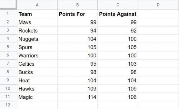
1. Suppose I have the following dataset and want to highlight cells of the team column where corresponding values in the “points for” and “points against” columns are not equal.
   
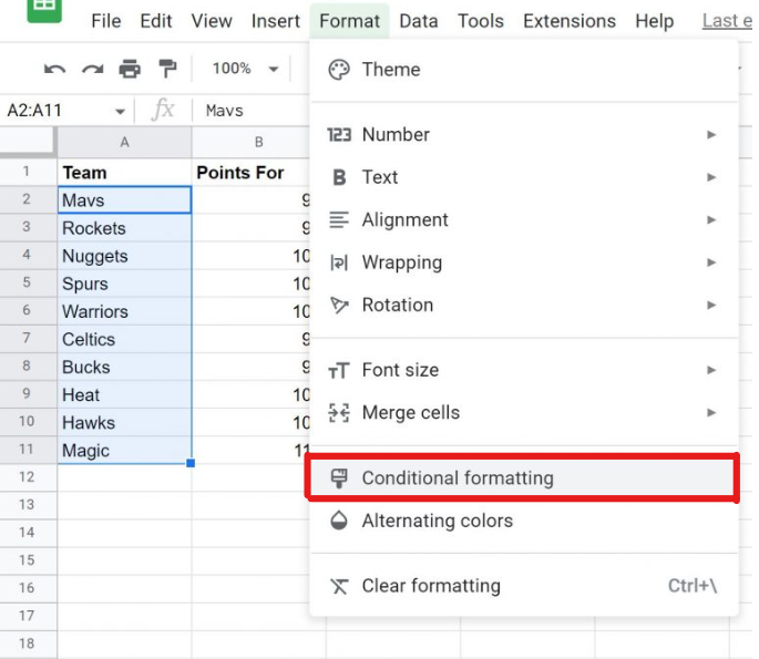
2. For that, select the cells you want to highlight (here, A2:A11) and click Format > Conditional Formatting.
   
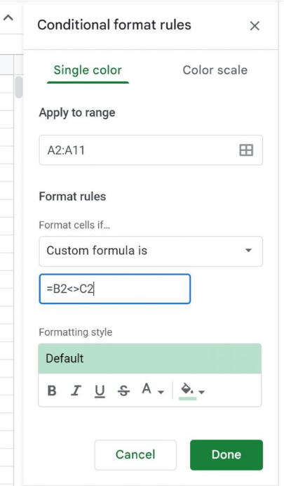
3. In the “conditional formatting rules” panel, click the “Format cells if” option, and in the dropdown menu, select “Custom formula is.” Then write the following formula: =B2<>C2.
   
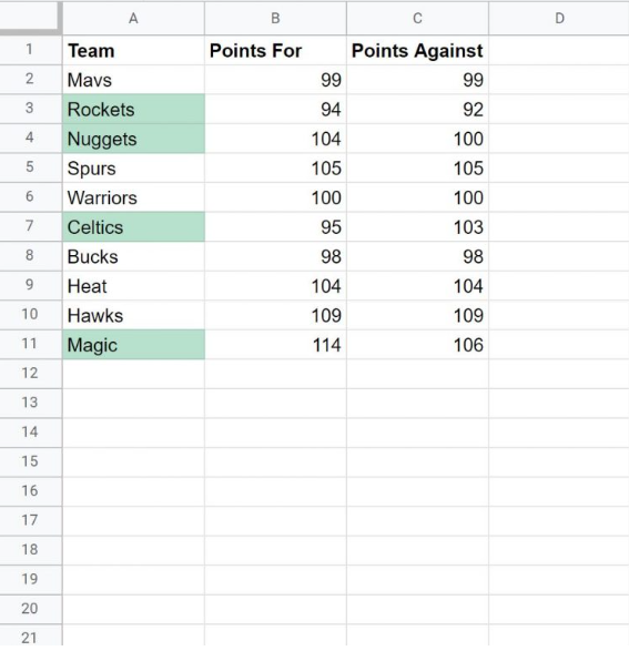
4. Then, click Done. The cells in Points for & Points against columns where corresponding values are not equal are highlighted.
   

By default, Google Sheets uses a light green background as a conditional formatting style. You can change the style any way you want.

Alternative: Not Equal Function (NE)

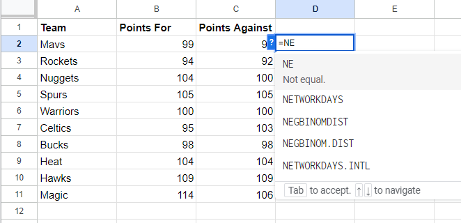
In place of Not Equal symbol, you can use the NE function to compare two values and to check if a value is present in the cell. 

1. Basic Comparison

1. In the adjacent empty cell, put the NE syntax.
   
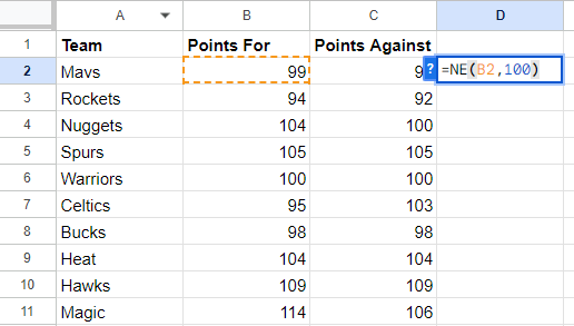
2. In a bracket, input the cells you want to compare. In my case, it’s B2 and C2.
   
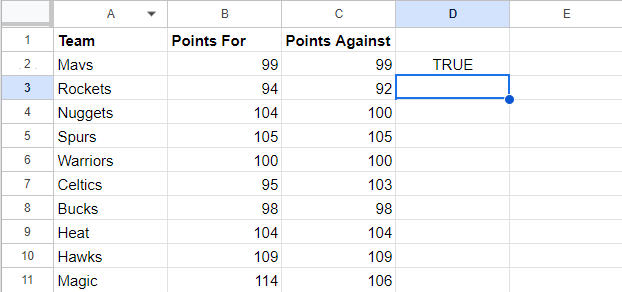
3. Press Enter.
   
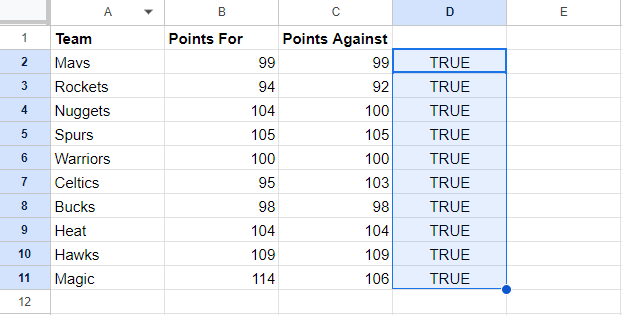
4. Copy it down to apply the formula to other cells.
   

2. Check cells containing a particular value

In this example, I will use the NE syntax to determine if a particular value is present in the cell or not.

Here’s how to do it:

1. In the empty cell next to the data set, input the NE syntax.
2. Then, in a bracket, input the cell you want to evaluate, followed by the data.
3. Then press Enter and copy the formula to the cells below. If data matches the value of cell, the result will be FALSE and, otherwise, TRUE.

Tips and Best Practices

• Try using the “Not equal” function in conditional formatting to highlight the ranges or cells based on certain applied conditions. It helps in better visualization of data and makes your life much easier.
• Combine “Not equal” with other functions like “SUMIF,” “COUNTIF,” “FILTER,” and others to create more complex formulas and ensure faster and better data analysis.
• Pay attention when writing formulas, and ensure they’re written and structured properly to get the desired result. Also, test them before applying them in practical scenarios. 
• Document your formulas, especially when using the “Not equal” syntax to make it easier for others to understand the logic and apply it correctly.
• If you have formulas that may return errors when their values change, you can use Google Sheets’ IFERROR function to handle them.

Frequently Asked Questions

Wrap Up!

With that comes an end to my guide. You now have step-by-step instructions on how to use the not-equal function and analyze the data more efficiently. Ensure not to miss anything when using them in combination with other functions.

Saying that, I’d like to bid adieu. I’ll see you in another such informational guide. Till then, goodbye and take care!