How To Add Alternate Row Color in Google Sheets?

There is something about colors and symmetry that makes regular sheets a lot more appealing. If done right, alternating row colors can help you attain that focus you want your clients to have on certain data points.

At times we have a data set that rationally compares two consecutive series of data. In that case, we need to not only enhance the data visually but distinguish them with the same symmetry and uniform color coding.

Luckily, you can use the same color for our rows but in an alternating manner. Learn how to use this to your benefit.

Ways To Alternating Colors in Google Sheets

You can, of course, color all your columns and rows. But there is a built-in feature that allows you to use the same color for alternate rows. Moreover, you can also make this type of color coding as your default setting for coloring.

Now here are three most prominent methods to add color to every other row in your Google Sheets.

Method 1: Using Format

1. Open the sheet.
2. Select the range of cells (rows and columns) where you want to apply the same color for alternate rows.
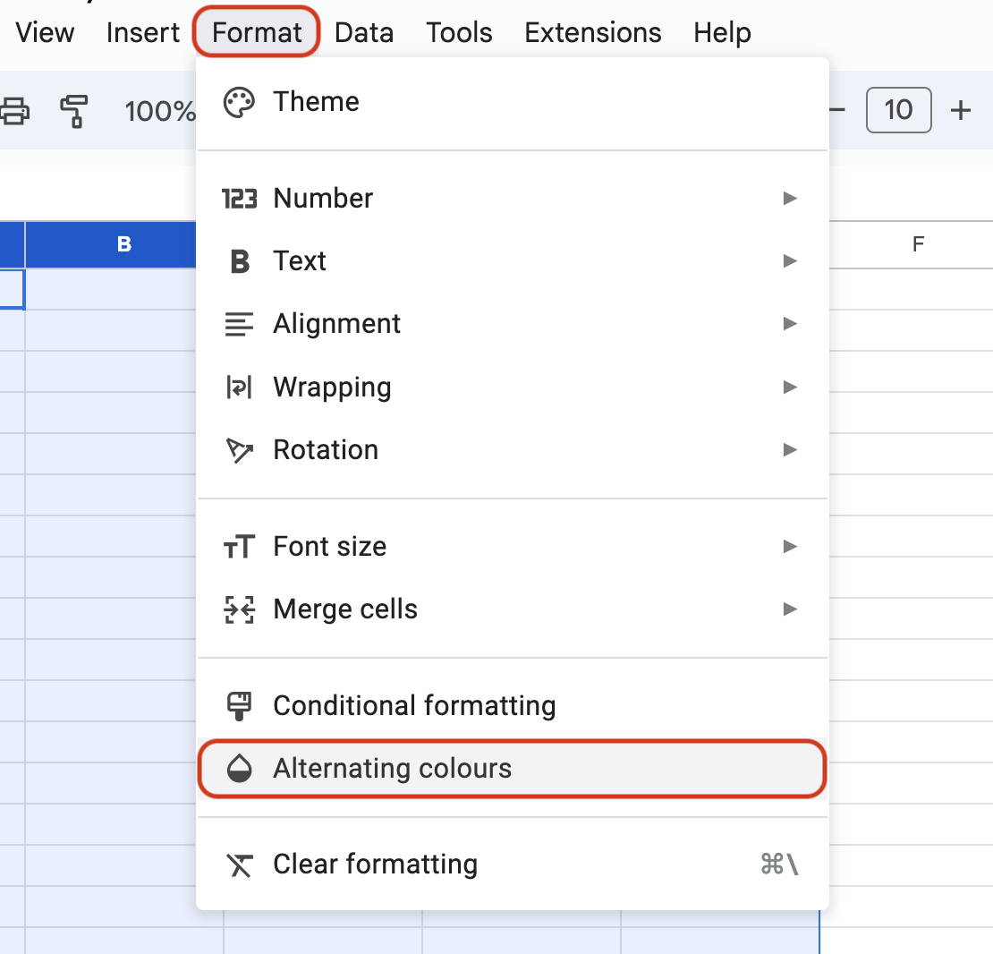
3. Go to “Format” tab from the main menu.
4. Select “Alternating colors” from the dropdown.

Method 2: Using Fill Color

1. Open the Google Sheets file where you want to add color to alternate rows.
2. Select the range of cells (rows and columns) where you want to apply the same color for alternate rows.
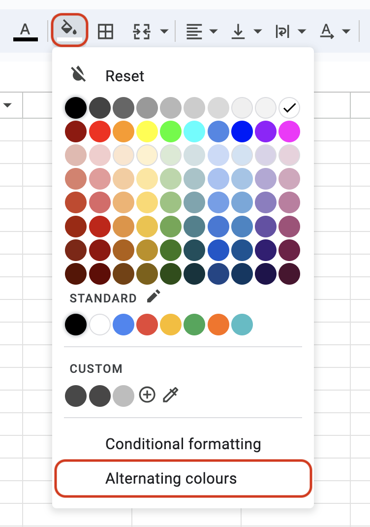
3. Go to “Fill color” from the Ribbon menu.
4. Select “Alternating colors” from the dropdown.

Method 3: Using Conditional Formatting

Now let us assume you want to use different colors for different rows but not in an alternating manner. You could use a condition for rows, and every row that matches that condition gets formatting.

For instance, if you want to color the even rows, then you can use the ISEVEN function. Here is a step-by-step process:

1. Open the sheet file.
2. Select the range of cells (rows and columns).
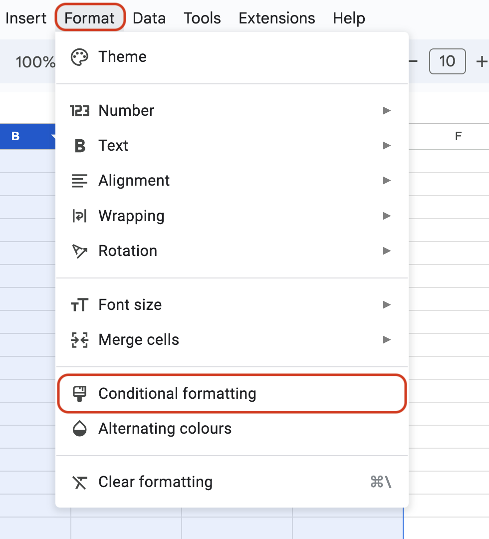
3. Go to “Format” from the main menu.
4. Select “Conditional formatting” from the menu.
5. Alternatively, you can also go to “Fill color” from the ribbon menu and select “Conditional formatting” from the dropdown.
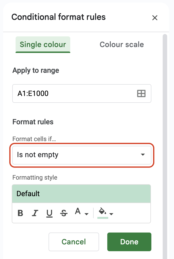
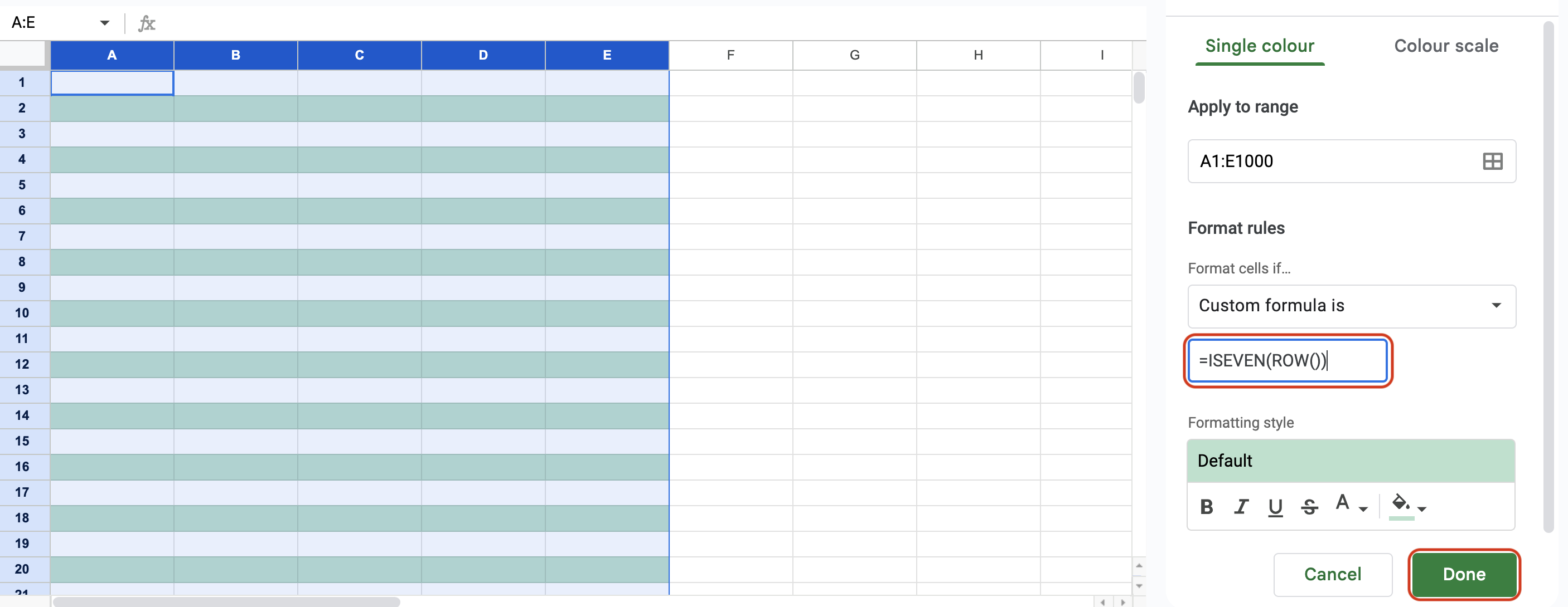
6. In the new editor that opens on the right side of the screen, choose the formula from the “format cells if…” dropdown from the format rules tab.
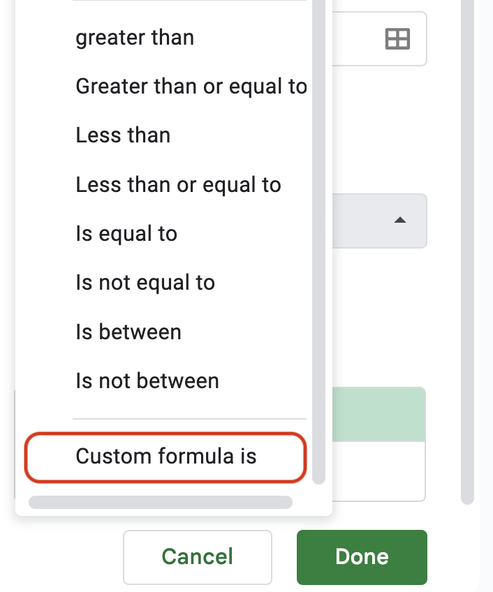
7. Select the rule you want to apply or select the “Custom formula” option.
8. Write down a custom formula with a function. For instance, if you want all the even rows to be colored, then write =ISEVEN(ROW()). This will check if the row is even, and if it is, then it will apply the formatting.
9. Click on “Done”.

That is it. Now you have put a condition, and upon matching that condition, Google Sheets will paint the rows with the color you have selected.

Choosing a Default Option

Google Sheets offers a range of different appealing color coding. You can choose the one you like or customize it yourself.

We will get to customizing the colors in a while, but before that, let’s take a look at how to set a default style for coloring.

The steps are in continuation of the above section where you have already applied the “Alternating colors” feature.

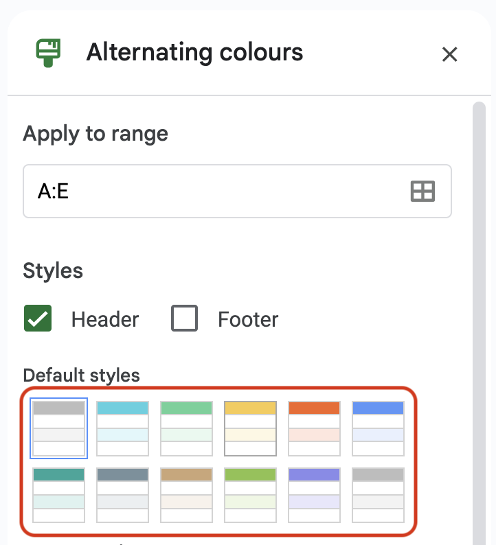
1. Find the editor on the right side of the screen upon applying “Alternating colors”.
2. Find the second tab in the editor with the heading “Styles”.
3. Select whether you want the header or footer to have the default style.
4. Now select from the 12 predesigned “Default styles” of color combinations and click on “Done”.
   

Done! Now every time you apply this feature of adding color to every other row, Google Sheets will use your default style of colors.

Customizing Color Style

Let’s assume you are either not happy with the “Default styles”, or you want to use a particular custom color in your sheets.

In that case, you have to access the next tab in the colors editor (which stays on the right side of the screen).

Here are the steps to apply custom colors to your rows (in continuation of the steps from the above section)

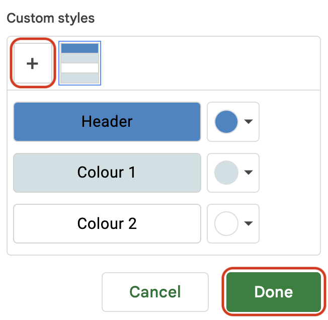
1. Scroll down in the editor and find the “Custom Styles” tab.
2. Now choose colors individually for the Header, Color 1, and Color 2.
3. Click the “+” sign above the “Default styles” to add it to the default and click on “Done”.
   

Not only alter colors but you can also make text autofit, merge cells, underline a text and do other customizations to organize your Google Sheets better.

Frequently Asked Questions

Wrap Up!

Alternating colors are great, and they visually enhance your tables. Exploring the color combinations and conditional formatting takes it to a completely different level. If your datasets are numerics, then you can have different colors based on the data values as well.