Date and time can sometimes appear in the same cell. The problem with this is that they both appear in different formats, and we may lose precious value while editing them. This is very common when you import sheets from other platforms.
Fortunately, it is possible to split the date and time in Excel, and there are two prominent methods to do it. And if you’re a nerd like me, you can also use VBA to write custom codes to execute custom commands.
Now, without further delay, let’s get into it!
Method 1: Using INT Function
The INT function denotes extracting the integer part in a cell’s value. MS Excel stores every value that is in the form of a date as a particular number.
So, if you use the INT function, it tells the sheet to extract the integer part from the cell and leave out other values.
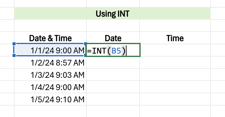
The syntax for the INT function is: =INT(cell address), where you have to mention the cell number in the brackets simply.
Given that all the date and time values are entered in a combined manner across a range of cells in a column, here is how you can separate them:
- Enter all the source data (date and time combined) in one range of a column.
- Now go to the adjacent cell to the first cell of the range.
- Enter this syntax: INT(cell address).
- Now press Enter, and the date will be displayed.
- Drag and drop the formula to apply the formula to the following cells.
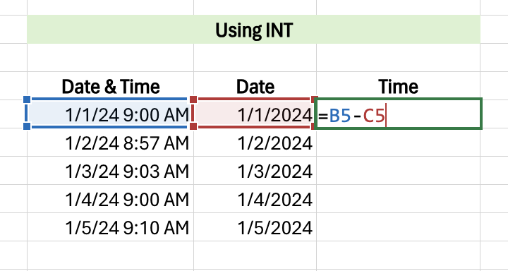
- For time apply the formula =B5-C5 (combined data cell – date data cell) and press enter.
Drag the formula, and the following cells will be filled with the time separately.
Method 2: Using Flash Fill Feature
Flash Fill is built to identify a certain pattern once you manually enter the data to a corresponding (or adjoining) cell.
Here is how you can use it for separating date and time values in a worksheet:
- Enter all the source data (date and time combined) in one range of a column.
- Now go to the adjacent cell to the first cell of the range.
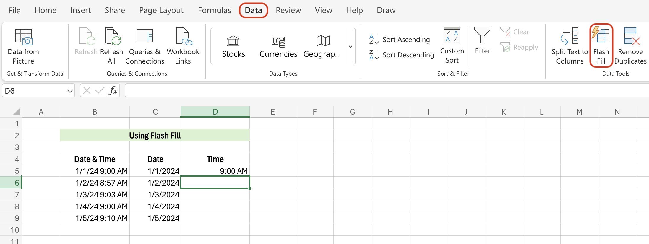
- Separate the date and time and enter the values manually.
- Press the Enter key, which will take you to the cell below, which is also an adjacent cell to the second cell of the range.
- Go to Fill from the ribbon menu and select “Flash Fill”.
- Alternatively, you can press Ctrl + E, which triggers the “Flash Fill”.
This will repeat the previously performed steps, which are to source values from adjacent cells and separate date and time. Note that Flash Fill tries to identify the pattern but may show inconsistency or inaccuracy at times.
Bonus Tip: If you have imported sheets, you may have many unnecessary hyphens. Here’s how to remove them.
Method 3: Using VBA
Visual Basic for Applications is a programming language that allows you to create programs that automate repetitive tasks in Excel. All you have to do is to create macros. These macros are in the form of instructions that trigger when repetitive tasks are detected.
You need to write these macros in a coding language. Once you write that code where you distinguish values and run the application, it automatically separates the values and enters them in different cells.
P.S. You can also use VBA to strikethrough in Excel.
Frequently Asked Questions
Yes, you can. Select the range of input data and go to the “Data Tools” option under the “Data” tab. Select “Text to Columns”, select the file type as “Delimited” from the pop-up, and select “Next”. Select “Space” as the delimiter in the next menu and click “Finish”.
Wrap Up!
If you have a couple of cells with date & time combined, the best way probably is the “Flash Fill” one. But if you have repeated entries in multiple sheets (due to imported files), then it is best to use the custom formula of INT.
Not to forget, you can also subtract time or days from two consecutive cells containing time or dates, but that is another topic for another day.


Leave a Reply